
Portal:Mathematics
The Mathematics Portal

Mathematics is the study of representing and reasoning about abstract objects (such as numbers, points, spaces, sets, structures, and games). Mathematics is used throughout the world as an essential tool in many fields, including natural science, engineering, medicine, and the social sciences. Applied mathematics, the branch of mathematics concerned with application of mathematical knowledge to other fields, inspires and makes use of new mathematical discoveries and sometimes leads to the development of entirely new mathematical disciplines, such as statistics and game theory. Mathematicians also engage in pure mathematics, or mathematics for its own sake, without having any application in mind. There is no clear line separating pure and applied mathematics, and practical applications for what began as pure mathematics are often discovered. (Full article...)
Featured articles –
-
 In algebraic geometry and theoretical physics, mirror symmetry is a relationship between geometric objects called Calabi–Yau manifolds. The term refers to a situation where two Calabi–Yau manifolds look very different geometrically but are nevertheless equivalent when employed as extra dimensions of string theory.
Early cases of mirror symmetry were discovered by physicists. Mathematicians became interested in this relationship around 1990 when Philip Candelas, Xenia de la Ossa, Paul Green, and Linda Parkes showed that it could be used as a tool in enumerative geometry, a branch of mathematics concerned with counting the number of solutions to geometric questions. Candelas and his collaborators showed that mirror symmetry could be used to count rational curves on a Calabi–Yau manifold, thus solving a longstanding problem. Although the original approach to mirror symmetry was based on physical ideas that were not understood in a mathematically precise way, some of its mathematical predictions have since been proven rigorously. (Full article...) -
The Quine–Putnam indispensability argument is an argument in the philosophy of mathematics for the existence of abstract mathematical objects such as numbers and sets, a position known as mathematical platonism. It was named after the philosophers Willard Quine and Hilary Putnam, and is one of the most important arguments in the philosophy of mathematics.
Although elements of the indispensability argument may have originated with thinkers such as Gottlob Frege and Kurt Gödel, Quine's development of the argument was unique for introducing to it a number of his philosophical positions such as naturalism, confirmational holism, and the criterion of ontological commitment. Putnam gave Quine's argument its first detailed formulation in his 1971 book Philosophy of Logic. He later came to disagree with various aspects of Quine's thinking, however, and formulated his own indispensability argument based on the no miracles argument in the philosophy of science. A standard form of the argument in contemporary philosophy is credited to Mark Colyvan; whilst being influenced by both Quine and Putnam, it differs in important ways from their formulations. It is presented in the Stanford Encyclopedia of Philosophy: (Full article...) -
The number π (/paɪ/; spelled out as "pi") is a mathematical constant that is the ratio of a circle's circumference to its diameter, approximately equal to 3.14159. The number π appears in many formulae across mathematics and physics. It is an irrational number, meaning that it cannot be expressed exactly as a ratio of two integers, although fractions such as are commonly used to approximate it. Consequently, its decimal representation never ends, nor enters a permanently repeating pattern. It is a transcendental number, meaning that it cannot be a solution of an equation involving only finite sums, products, powers, and integers. The transcendence of π implies that it is impossible to solve the ancient challenge of squaring the circle with a compass and straightedge. The decimal digits of π appear to be randomly distributed, but no proof of this conjecture has been found.
For thousands of years, mathematicians have attempted to extend their understanding of π, sometimes by computing its value to a high degree of accuracy. Ancient civilizations, including the Egyptians and Babylonians, required fairly accurate approximations of π for practical computations. Around 250 BC, the Greek mathematician Archimedes created an algorithm to approximate π with arbitrary accuracy. In the 5th century AD, Chinese mathematicians approximated π to seven digits, while Indian mathematicians made a five-digit approximation, both using geometrical techniques. The first computational formula for π, based on infinite series, was discovered a millennium later. The earliest known use of the Greek letter π to represent the ratio of a circle's circumference to its diameter was by the Welsh mathematician William Jones in 1706. (Full article...) -

Josiah Willard Gibbs (/ɡɪbz/; February 11, 1839 – April 28, 1903) was an American scientist who made significant theoretical contributions to physics, chemistry, and mathematics. His work on the applications of thermodynamics was instrumental in transforming physical chemistry into a rigorous deductive science. Together with James Clerk Maxwell and Ludwig Boltzmann, he created statistical mechanics (a term that he coined), explaining the laws of thermodynamics as consequences of the statistical properties of ensembles of the possible states of a physical system composed of many particles. Gibbs also worked on the application of Maxwell's equations to problems in physical optics. As a mathematician, he created modern vector calculus (independently of the British scientist Oliver Heaviside, who carried out similar work during the same period) and described the Gibbs phenomenon in the theory of Fourier analysis.
In 1863, Yale University awarded Gibbs the first American doctorate in engineering. After a three-year sojourn in Europe, Gibbs spent the rest of his career at Yale, where he was a professor of mathematical physics from 1871 until his death in 1903. Working in relative isolation, he became the earliest theoretical scientist in the United States to earn an international reputation and was praised by Albert Einstein as "the greatest mind in American history." In 1901, Gibbs received what was then considered the highest honor awarded by the international scientific community, the Copley Medal of the Royal Society of London, "for his contributions to mathematical physics." (Full article...) -
Zhang Heng (Chinese: 張衡; AD 78–139), formerly romanized Chang Heng, was a Chinese polymathic scientist and statesman who lived during the Han dynasty. Educated in the capital cities of Luoyang and Chang'an, he achieved success as an astronomer, mathematician, seismologist, hydraulic engineer, inventor, geographer, cartographer, ethnographer, artist, poet, philosopher, politician, and literary scholar.
Zhang Heng began his career as a minor civil servant in Nanyang. Eventually, he became Chief Astronomer, Prefect of the Majors for Official Carriages, and then Palace Attendant at the imperial court. His uncompromising stance on historical and calendrical issues led to his becoming a controversial figure, preventing him from rising to the status of Grand Historian. His political rivalry with the palace eunuchs during the reign of Emperor Shun (r. 125–144) led to his decision to retire from the central court to serve as an administrator of Hejian Kingdom in present-day Hebei. Zhang returned home to Nanyang for a short time, before being recalled to serve in the capital once more in 138. He died there a year later, in 139. (Full article...) -
Amalie Emmy Noether (US: /ˈnʌtər/, UK: /ˈnɜːtə/; German: [ˈnøːtɐ]; 23 March 1882 – 14 April 1935) was a German mathematician who made many important contributions to abstract algebra. She proved Noether's first and second theorems, which are fundamental in mathematical physics. She was described by Pavel Alexandrov, Albert Einstein, Jean Dieudonné, Hermann Weyl and Norbert Wiener as the most important woman in the history of mathematics. As one of the leading mathematicians of her time, she developed theories of rings, fields, and algebras. In physics, Noether's theorem explains the connection between symmetry and conservation laws.
Noether was born to a Jewish family in the Franconian town of Erlangen; her father was the mathematician Max Noether. She originally planned to teach French and English after passing the required examinations but instead studied mathematics at the University of Erlangen, where her father lectured. After completing her doctorate in 1907 under the supervision of Paul Gordan, she worked at the Mathematical Institute of Erlangen without pay for seven years. At the time, women were largely excluded from academic positions. In 1915, she was invited by David Hilbert and Felix Klein to join the mathematics department at the University of Göttingen, a world-renowned center of mathematical research. The philosophical faculty objected, however, and she spent four years lecturing under Hilbert's name. Her habilitation was approved in 1919, allowing her to obtain the rank of Privatdozent. (Full article...) -
General relativity, also known as the general theory of relativity and Einstein's theory of gravity, is the geometric theory of gravitation published by Albert Einstein in 1915 and is the current description of gravitation in modern physics. General relativity generalizes special relativity and refines Newton's law of universal gravitation, providing a unified description of gravity as a geometric property of space and time or four-dimensional spacetime. In particular, the curvature of spacetime is directly related to the energy and momentum of whatever matter and radiation are present. The relation is specified by the Einstein field equations, a system of second order partial differential equations.
Newton's law of universal gravitation, which describes classical gravity, can be seen as a prediction of general relativity for the almost flat spacetime geometry around stationary mass distributions. Some predictions of general relativity, however, are beyond Newton's law of universal gravitation in classical physics. These predictions concern the passage of time, the geometry of space, the motion of bodies in free fall, and the propagation of light, and include gravitational time dilation, gravitational lensing, the gravitational redshift of light, the Shapiro time delay and singularities/black holes. So far, all tests of general relativity have been shown to be in agreement with the theory. The time-dependent solutions of general relativity enable us to talk about the history of the universe and have provided the modern framework for cosmology, thus leading to the discovery of the Big Bang and cosmic microwave background radiation. Despite the introduction of a number of alternative theories, general relativity continues to be the simplest theory consistent with experimental data. (Full article...) -
In classical mechanics, the Laplace–Runge–Lenz (LRL) vector is a vector used chiefly to describe the shape and orientation of the orbit of one astronomical body around another, such as a binary star or a planet revolving around a star. For two bodies interacting by Newtonian gravity, the LRL vector is a constant of motion, meaning that it is the same no matter where it is calculated on the orbit; equivalently, the LRL vector is said to be conserved. More generally, the LRL vector is conserved in all problems in which two bodies interact by a central force that varies as the inverse square of the distance between them; such problems are called Kepler problems.
The hydrogen atom is a Kepler problem, since it comprises two charged particles interacting by Coulomb's law of electrostatics, another inverse-square central force. The LRL vector was essential in the first quantum mechanical derivation of the spectrum of the hydrogen atom, before the development of the Schrödinger equation. However, this approach is rarely used today. (Full article...) -
Marian Adam Rejewski (Polish: [ˈmarjan rɛˈjɛfskʲi] ⓘ; 16 August 1905 – 13 February 1980) was a Polish mathematician and cryptologist who in late 1932 reconstructed the sight-unseen German military Enigma cipher machine, aided by limited documents obtained by French military intelligence.
Over the next nearly seven years, Rejewski and fellow mathematician-cryptologists Jerzy Różycki and Henryk Zygalski, working at the Polish General Staff's Cipher Bureau, developed techniques and equipment for decrypting the Enigma ciphers, even as the Germans introduced modifications to their Enigma machines and encryption procedures. Rejewski's contributions included the cryptologic card catalog and the cryptologic bomb. (Full article...) -
Georg Ferdinand Ludwig Philipp Cantor (/ˈkæntɔːr/ KAN-tor, German: [ˈɡeːɔʁk ˈfɛʁdinant ˈluːtvɪç ˈfiːlɪp ˈkantoːɐ̯]; 3 March [O.S. 19 February] 1845 – 6 January 1918) was a mathematician who played a pivotal role in the creation of set theory, which has become a fundamental theory in mathematics. Cantor established the importance of one-to-one correspondence between the members of two sets, defined infinite and well-ordered sets, and proved that the real numbers are more numerous than the natural numbers. Cantor's method of proof of this theorem implies the existence of an infinity of infinities. He defined the cardinal and ordinal numbers and their arithmetic. Cantor's work is of great philosophical interest, a fact he was well aware of.
Originally, Cantor's theory of transfinite numbers was regarded as counter-intuitive – even shocking. This caused it to encounter resistance from mathematical contemporaries such as Leopold Kronecker and Henri Poincaré and later from Hermann Weyl and L. E. J. Brouwer, while Ludwig Wittgenstein raised philosophical objections; see Controversy over Cantor's theory. Cantor, a devout Lutheran Christian, believed the theory had been communicated to him by God. Some Christian theologians (particularly neo-Scholastics) saw Cantor's work as a challenge to the uniqueness of the absolute infinity in the nature of God – on one occasion equating the theory of transfinite numbers with pantheism – a proposition that Cantor vigorously rejected. Not all theologians were against Cantor's theory; prominent neo-scholastic philosopher Constantin Gutberlet was in favor of it and Cardinal Johann Baptist Franzelin accepted it as a valid theory (after Cantor made some important clarifications). (Full article...) -
Robert Hues (1553 – 24 May 1632) was an English mathematician and geographer. He attended St. Mary Hall at Oxford, and graduated in 1578. Hues became interested in geography and mathematics, and studied navigation at a school set up by Walter Raleigh. During a trip to Newfoundland, he made observations which caused him to doubt the accepted published values for variations of the compass. Between 1586 and 1588, Hues travelled with Thomas Cavendish on a circumnavigation of the globe, performing astronomical observations and taking the latitudes of places they visited. Beginning in August 1591, Hues and Cavendish again set out on another circumnavigation of the globe. During the voyage, Hues made astronomical observations in the South Atlantic, and continued his observations of the variation of the compass at various latitudes and at the Equator. Cavendish died on the journey in 1592, and Hues returned to England the following year.
In 1594, Hues published his discoveries in the Latin work Tractatus de globis et eorum usu (Treatise on Globes and Their Use) which was written to explain the use of the terrestrial and celestial globes that had been made and published by Emery Molyneux in late 1592 or early 1593, and to encourage English sailors to use practical astronomical navigation. Hues' work subsequently went into at least 12 other printings in Dutch, English, French and Latin. (Full article...) -

The regular triangular tiling of the plane, whose symmetries are described by the affine symmetric group S̃3
The affine symmetric groups are a family of mathematical structures that describe the symmetries of the number line and the regular triangular tiling of the plane, as well as related higher-dimensional objects. In addition to this geometric description, the affine symmetric groups may be defined in other ways: as collections of permutations (rearrangements) of the integers (..., −2, −1, 0, 1, 2, ...) that are periodic in a certain sense, or in purely algebraic terms as a group with certain generators and relations. They are studied in combinatorics and representation theory.
A finite symmetric group consists of all permutations of a finite set. Each affine symmetric group is an infinite extension of a finite symmetric group. Many important combinatorial properties of the finite symmetric groups can be extended to the corresponding affine symmetric groups. Permutation statistics such as descents and inversions can be defined in the affine case. As in the finite case, the natural combinatorial definitions for these statistics also have a geometric interpretation. (Full article...) -
Leonhard Euler (/ˈɔɪlər/ OY-lər, German: [ˈleːɔnhaʁt ˈʔɔʏlɐ] ⓘ, Swiss Standard German: [ˈleːɔnhart ˈɔʏlər]; 15 April 1707 – 18 September 1783) was a Swiss mathematician, physicist, astronomer, geographer, logician, and engineer who founded the studies of graph theory and topology and made pioneering and influential discoveries in many other branches of mathematics such as analytic number theory, complex analysis, and infinitesimal calculus. He introduced much of modern mathematical terminology and notation, including the notion of a mathematical function. He is also known for his work in mechanics, fluid dynamics, optics, astronomy, and music theory.
Euler is held to be one of the greatest mathematicians in history and the greatest of the 18th century. Several great mathematicians who produced their work after Euler's death have recognised his importance in the field as shown by quotes attributed to many of them: Pierre-Simon Laplace expressed Euler's influence on mathematics by stating, "Read Euler, read Euler, he is the master of us all." Carl Friedrich Gauss wrote: "The study of Euler's works will remain the best school for the different fields of mathematics, and nothing else can replace it." Euler is also widely considered to be the most prolific; his 866 publications as well as his correspondences are being collected in the Opera Omnia Leonhard Euler which, when completed, will consist of 81 quarto volumes. He spent most of his adult life in Saint Petersburg, Russia, and in Berlin, then the capital of Prussia. (Full article...) -
Archimedes of Syracuse (/ˌɑːrkɪˈmiːdiːz/ AR-kim-EE-deez; c. 287 – c. 212 BC) was an Ancient Greek mathematician, physicist, engineer, astronomer, and inventor from the ancient city of Syracuse in Sicily. Although few details of his life are known, he is regarded as one of the leading scientists in classical antiquity. Considered the greatest mathematician of ancient history, and one of the greatest of all time, Archimedes anticipated modern calculus and analysis by applying the concept of the infinitely small and the method of exhaustion to derive and rigorously prove a range of geometrical theorems. These include the area of a circle, the surface area and volume of a sphere, the area of an ellipse, the area under a parabola, the volume of a segment of a paraboloid of revolution, the volume of a segment of a hyperboloid of revolution, and the area of a spiral.
Archimedes' other mathematical achievements include deriving an approximation of pi, defining and investigating the Archimedean spiral, and devising a system using exponentiation for expressing very large numbers. He was also one of the first to apply mathematics to physical phenomena, working on statics and hydrostatics. Archimedes' achievements in this area include a proof of the law of the lever, the widespread use of the concept of center of gravity, and the enunciation of the law of buoyancy known as Archimedes' principle. He is also credited with designing innovative machines, such as his screw pump, compound pulleys, and defensive war machines to protect his native Syracuse from invasion. (Full article...) -

Stylistic impression of the number, representing how its decimals go on infinitely
In mathematics, 0.999... (also written as 0.9, 0. or 0.(9)) is a notation for the repeating decimal consisting of an unending sequence of 9s after the decimal point. This repeating decimal is a numeral that represents the smallest number no less than every number in the sequence ; that is, the supremum of this sequence. This number is equal to 1. In other words, "0.999..." is not "almost exactly 1" or "very, very nearly but not quite 1"; rather, "0.999..." and "1" represent exactly the same number.
There are many ways of showing this equality, from intuitive arguments to mathematically rigorous proofs. The technique used depends on the target audience, background assumptions, historical context, and preferred development of the real numbers, the system within which 0.999... is commonly defined. In other systems, 0.999... can have the same meaning, a different definition, or be undefined. (Full article...)


.jpg)


Selected image –

Good articles –
-
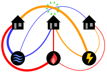
Diagram of the three utilities problem showing lines in a plane. Can each house be connected to each utility, with no connection lines crossing?
The classical mathematical puzzle known as the three utilities problem or sometimes water, gas and electricity asks for non-crossing connections to be drawn between three houses and three utility companies in the plane. When posing it in the early 20th century, Henry Dudeney wrote that it was already an old problem. It is an impossible puzzle: it is not possible to connect all nine lines without crossing. Versions of the problem on nonplanar surfaces such as a torus or Möbius strip, or that allow connections to pass through other houses or utilities, can be solved.
This puzzle can be formalized as a problem in topological graph theory by asking whether the complete bipartite graph , with vertices representing the houses and utilities and edges representing their connections, has a graph embedding in the plane. The impossibility of the puzzle corresponds to the fact that is not a planar graph. Multiple proofs of this impossibility are known, and form part of the proof of Kuratowski's theorem characterizing planar graphs by two forbidden subgraphs, one of which is . The question of minimizing the number of crossings in drawings of complete bipartite graphs is known as Turán's brick factory problem, and for the minimum number of crossings is one. (Full article...) -

Measuring the width of a Reuleaux triangle as the distance between parallel supporting lines. Because this distance does not depend on the direction of the lines, the Reuleaux triangle is a curve of constant width.
In geometry, a curve of constant width is a simple closed curve in the plane whose width (the distance between parallel supporting lines) is the same in all directions. The shape bounded by a curve of constant width is a body of constant width or an orbiform, the name given to these shapes by Leonhard Euler. Standard examples are the circle and the Reuleaux triangle. These curves can also be constructed using circular arcs centered at crossings of an arrangement of lines, as the involutes of certain curves, or by intersecting circles centered on a partial curve.
Every body of constant width is a convex set, its boundary crossed at most twice by any line, and if the line crosses perpendicularly it does so at both crossings, separated by the width. By Barbier's theorem, the body's perimeter is exactly π times its width, but its area depends on its shape, with the Reuleaux triangle having the smallest possible area for its width and the circle the largest. Every superset of a body of constant width includes pairs of points that are farther apart than the width, and every curve of constant width includes at least six points of extreme curvature. Although the Reuleaux triangle is not smooth, curves of constant width can always be approximated arbitrarily closely by smooth curves of the same constant width. (Full article...) -
In mathematics, the three-gap theorem, three-distance theorem, or Steinhaus conjecture states that if one places n points on a circle, at angles of θ, 2θ, 3θ, ... from the starting point, then there will be at most three distinct distances between pairs of points in adjacent positions around the circle. When there are three distances, the largest of the three always equals the sum of the other two. Unless θ is a rational multiple of π, there will also be at least two distinct distances.
This result was conjectured by Hugo Steinhaus, and proved in the 1950s by Vera T. Sós, János Surányi, and Stanisław Świerczkowski; more proofs were added by others later. Applications of the three-gap theorem include the study of plant growth and musical tuning systems, and the theory of light reflection within a mirrored square. (Full article...) -
In geometry, the Dehn invariant is a value used to determine whether one polyhedron can be cut into pieces and reassembled ("dissected") into another, and whether a polyhedron or its dissections can tile space. It is named after Max Dehn, who used it to solve Hilbert's third problem by proving that not all polyhedra with equal volume could be dissected into each other.
Two polyhedra have a dissection into polyhedral pieces that can be reassembled into either one, if and only if their volumes and Dehn invariants are equal. Having Dehn invariant zero is a necessary (but not sufficient) condition for being a space-filling polyhedron, and a polyhedron can be cut up and reassembled into a space-filling polyhedron if and only if its Dehn invariant is zero. The Dehn invariant of a self-intersection-free flexible polyhedron is invariant as it flexes. Dehn invariants are also an invariant for dissection in higher dimensions, and (with volume) a complete invariant in four dimensions. (Full article...) -

A homomorphism from the flower snark J5 into the cycle graph C5.
It is also a retraction onto the subgraph on the central five vertices. Thus J5 is in fact homomorphically equivalent to the core C5.
In the mathematical field of graph theory, a graph homomorphism is a mapping between two graphs that respects their structure. More concretely, it is a function between the vertex sets of two graphs that maps adjacent vertices to adjacent vertices.
Homomorphisms generalize various notions of graph colorings and allow the expression of an important class of constraint satisfaction problems, such as certain scheduling or frequency assignment problems.
The fact that homomorphisms can be composed leads to rich algebraic structures: a preorder on graphs, a distributive lattice, and a category (one for undirected graphs and one for directed graphs).
The computational complexity of finding a homomorphism between given graphs is prohibitive in general, but a lot is known about special cases that are solvable in polynomial time. Boundaries between tractable and intractable cases have been an active area of research. (Full article...) -

Hendrik Antoon Lorentz (right) after whom the Lorentz group is named and Albert Einstein whose special theory of relativity is the main source of application. Photo taken by Paul Ehrenfest 1921.
The Lorentz group is a Lie group of symmetries of the spacetime of special relativity. This group can be realized as a collection of matrices, linear transformations, or unitary operators on some Hilbert space; it has a variety of representations. This group is significant because special relativity together with quantum mechanics are the two physical theories that are most thoroughly established, and the conjunction of these two theories is the study of the infinite-dimensional unitary representations of the Lorentz group. These have both historical importance in mainstream physics, as well as connections to more speculative present-day theories. (Full article...) -

Euclidean minimum spanning tree of 25 random points in the plane
A Euclidean minimum spanning tree of a finite set of points in the Euclidean plane or higher-dimensional Euclidean space connects the points by a system of line segments with the points as endpoints, minimizing the total length of the segments. In it, any two points can reach each other along a path through the line segments. It can be found as the minimum spanning tree of a complete graph with the points as vertices and the Euclidean distances between points as edge weights.
The edges of the minimum spanning tree meet at angles of at least 60°, at most six to a vertex. In higher dimensions, the number of edges per vertex is bounded by the kissing number of tangent unit spheres. The total length of the edges, for points in a unit square, is at most proportional to the square root of the number of points. Each edge lies in an empty region of the plane, and these regions can be used to prove that the Euclidean minimum spanning tree is a subgraph of other geometric graphs including the relative neighborhood graph and Delaunay triangulation. By constructing the Delaunay triangulation and then applying a graph minimum spanning tree algorithm, the minimum spanning tree of given planar points may be found in time , as expressed in big O notation. This is optimal in some models of computation, although faster randomized algorithms exist for points with integer coordinates. For points in higher dimensions, finding an optimal algorithm remains an open problem. (Full article...) -

Fig. 1: A binary search tree of size 9 and depth 3, with 8 at the root. The leaves are not drawn.
In computer science, a binary search tree (BST), also called an ordered or sorted binary tree, is a rooted binary tree data structure with the key of each internal node being greater than all the keys in the respective node's left subtree and less than the ones in its right subtree. The time complexity of operations on the binary search tree is linear with respect to the height of the tree.
Binary search trees allow binary search for fast lookup, addition, and removal of data items. Since the nodes in a BST are laid out so that each comparison skips about half of the remaining tree, the lookup performance is proportional to that of binary logarithm. BSTs were devised in the 1960s for the problem of efficient storage of labeled data and are attributed to Conway Berners-Lee and David Wheeler. (Full article...) -

Srinivasa Ramanujan
(22 December 1887 – 26 April 1920) was an Indian mathematician. Though he had almost no formal training in pure mathematics, he made substantial contributions to mathematical analysis, number theory, infinite series, and continued fractions, including solutions to mathematical problems then considered unsolvable.
Ramanujan initially developed his own mathematical research in isolation. According to Hans Eysenck, "he tried to interest the leading professional mathematicians in his work, but failed for the most part. What he had to show them was too novel, too unfamiliar, and additionally presented in unusual ways; they could not be bothered". Seeking mathematicians who could better understand his work, in 1913 he began a mail correspondence with the English mathematician G. H. Hardy at the University of Cambridge, England. Recognising Ramanujan's work as extraordinary, Hardy arranged for him to travel to Cambridge. In his notes, Hardy commented that Ramanujan had produced groundbreaking new theorems, including some that "defeated me completely; I had never seen anything in the least like them before", and some recently proven but highly advanced results. (Full article...) -
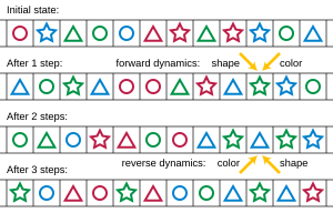
A one-dimensional reversible cellular automaton with nine states. At each step, each cell copies the shape from its left neighbor, and the color from its right neighbor.
A reversible cellular automaton is a cellular automaton in which every configuration has a unique predecessor. That is, it is a regular grid of cells, each containing a state drawn from a finite set of states, with a rule for updating all cells simultaneously based on the states of their neighbors, such that the previous state of any cell before an update can be determined uniquely from the updated states of all the cells. The time-reversed dynamics of a reversible cellular automaton can always be described by another cellular automaton rule, possibly on a much larger neighborhood.
Several methods are known for defining cellular automata rules that are reversible; these include the block cellular automaton method, in which each update partitions the cells into blocks and applies an invertible function separately to each block, and the second-order cellular automaton method, in which the update rule combines states from two previous steps of the automaton. When an automaton is not defined by one of these methods, but is instead given as a rule table, the problem of testing whether it is reversible is solvable for block cellular automata and for one-dimensional cellular automata, but is undecidable for other types of cellular automata. (Full article...) -

Four opaque sets for a unit square. Upper left: its boundary, length 4. Upper right: Three sides, length 3. Lower left: a Steiner tree of the vertices, length . Lower right: the conjectured optimal solution, length .
In discrete geometry, an opaque set is a system of curves or other set in the plane that blocks all lines of sight across a polygon, circle, or other shape. Opaque sets have also been called barriers, beam detectors, opaque covers, or (in cases where they have the form of a forest of line segments or other curves) opaque forests. Opaque sets were introduced by Stefan Mazurkiewicz in 1916, and the problem of minimizing their total length was posed by Frederick Bagemihl in 1959.
For instance, visibility through a unit square can be blocked by its four boundary edges, with length 4, but a shorter opaque forest blocks visibility across the square with length . It is unproven whether this is the shortest possible opaque set for the square, and for most other shapes this problem similarly remains unsolved. The shortest opaque set for any bounded convex set in the plane has length at most the perimeter of the set, and at least half the perimeter. For the square, a slightly stronger lower bound than half the perimeter is known. Another convex set whose opaque sets are commonly studied is the unit circle, for which the shortest connected opaque set has length . Without the assumption of connectivity, the shortest opaque set for the circle has length at least and at most . (Full article...) -
In mathematics, the Borromean rings are three simple closed curves in three-dimensional space that are topologically linked and cannot be separated from each other, but that break apart into two unknotted and unlinked loops when any one of the three is cut or removed. Most commonly, these rings are drawn as three circles in the plane, in the pattern of a Venn diagram, alternatingly crossing over and under each other at the points where they cross. Other triples of curves are said to form the Borromean rings as long as they are topologically equivalent to the curves depicted in this drawing.
The Borromean rings are named after the Italian House of Borromeo, who used the circular form of these rings as an element of their coat of arms, but designs based on the Borromean rings have been used in many cultures, including by the Norsemen and in Japan. They have been used in Christian symbolism as a sign of the Trinity, and in modern commerce as the logo of Ballantine beer, giving them the alternative name Ballantine rings. Physical instances of the Borromean rings have been made from linked DNA or other molecules, and they have analogues in the Efimov state and Borromean nuclei, both of which have three components bound to each other although no two of them are bound. (Full article...)


Did you know (auto-generated) –

- ... that a folded paper lantern shows that certain mathematical definitions of surface area are incorrect?
- ... that mathematician Mathias Metternich was one of the founders of the Jacobin club of the Republic of Mainz?
- ... that despite a mathematical model deeming the ice cream bar flavour Goody Goody Gum Drops impossible, it was still created?
- ... that after Archimedes first defined convex curves, mathematicians lost interest in their analysis until the 19th century, more than two millennia later?
- ... that mathematics professor Ari Nagel has fathered more than a hundred children?
- ... that more than 60 scientific papers authored by mathematician Paul Erdős were published posthumously?
- ... that Latvian-Soviet artist Karlis Johansons exhibited a skeletal tensegrity form of the Schönhardt polyhedron seven years before Erich Schönhardt's 1928 paper on its mathematics?
- ... that subgroup distortion theory, introduced by Misha Gromov in 1993, can help encode text?
More did you know –
- ...that Ostomachion is a mathematical treatise attributed to Archimedes on a 14-piece tiling puzzle similar to tangram?
- ...that some functions can be written as an infinite sum of trigonometric polynomials and that this sum is called the Fourier series of that function?
- ...that the identity elements for arithmetic operations make use of the only two whole numbers that are neither composites nor prime numbers, 0 and 1?
- ...that as of April 2010 only 35 even numbers have been found that are not the sum of two primes which are each in a Twin Primes pair? ref
- ...the Piphilology record (memorizing digits of Pi) is 70000 as of Mar 2015?
- ...that people are significantly slower to identify the parity of zero than other whole numbers, regardless of age, language spoken, or whether the symbol or word for zero is used?
- ...that Auction theory was successfully used in 1994 to sell FCC airwave spectrum, in a financial application of game theory?
Selected article –
 |
| A polar grid with several angles labeled Image credit: User:Mets501 |
The polar coordinate system is a two-dimensional coordinate system in which points are given by an angle and a distance from a central point known as the pole (equivalent to the origin in the more familiar Cartesian coordinate system). The polar coordinate system is used in many fields, including mathematics, physics, engineering, navigation and robotics. It is especially useful in situations where the relationship between two points is most easily expressed in terms of angles and distance; in the Cartesian coordinate system, such a relationship can only be found through trigonometric formulae. For many types of curves, a polar equation is the simplest means of representation of variables.
It is known that the Greeks used the concepts of angle and radius. The astronomer Hipparchus (190-120 BC) tabulated a table of chord functions giving the length of the chord for each angle, and there are references to his using polar coordinates in establishing stellar positions. (Full article...)
| View all selected articles |
Subcategories

Algebra | Arithmetic | Analysis | Complex analysis | Applied mathematics | Calculus | Category theory | Chaos theory | Combinatorics | Dynamical systems | Fractals | Game theory | Geometry | Algebraic geometry | Graph theory | Group theory | Linear algebra | Mathematical logic | Model theory | Multi-dimensional geometry | Number theory | Numerical analysis | Optimization | Order theory | Probability and statistics | Set theory | Statistics | Topology | Algebraic topology | Trigonometry | Linear programming
Mathematics | History of mathematics | Mathematicians | Awards | Education | Literature | Notation | Organizations | Theorems | Proofs | Unsolved problems
Topics in mathematics
| General | Foundations | Number theory | Discrete mathematics |
|---|---|---|---|
| |||
| Algebra | Analysis | Geometry and topology | Applied mathematics |
Index of mathematics articles
| ARTICLE INDEX: | |
| MATHEMATICIANS: |
Related portals
WikiProjects
![]() The Mathematics WikiProject is the center for mathematics-related editing on Wikipedia. Join the discussion on the project's talk page.
The Mathematics WikiProject is the center for mathematics-related editing on Wikipedia. Join the discussion on the project's talk page.
|
Project pages Essays Subprojects Related projects
|
Things you can do
|
In other Wikimedia projects
The following Wikimedia Foundation sister projects provide more on this subject:
-
 Commons
Free media repository -
 Wikibooks
Free textbooks and manuals -
 Wikidata
Free knowledge base -
 Wikinews
Free-content news -
 Wikiquote
Collection of quotations -
 Wikisource
Free-content library -
 Wikiversity
Free learning tools -
 Wiktionary
Dictionary and thesaurus


